Pipeline Stress Analysis Methodology
 Pipeline Stress Analysis Procedure
Below is a flowchart outlining the procedure for pipeline stress analysis.
- Information collection involves gathering the necessary input data for analysis. This includes the Design Basis Memorandum (DBM), which encompasses design codes and specifications, operating pressure and temperature, pipeline class locations, fluid details, and more. Additional information required are pipeline alignment sheets, piping isometrics, plot plans, pipes and fittings specifications, piping support drawings, mechanical equipment drawings and engineering data, process flow diagrams (PFD), geotechnical reports, and other relevant information.
- Modeling is to use analysis software to create stress analysis models based on the collected input data. The following factors are typically considered:
1) Model boundaries
The stress model should cover the entire section of the pipeline being analyzed and extend beyond the calculated Virtual Anchor Length (VAL) to minimize the impact of boundary conditions at both ends of the model. The VAL can be calculated as follows:

Where,
Cross section area of pipe
Coefficient of thermal expression
Axial soil spring stiffness
2) Pipe, fitting and support modeling
The pipe run is modeled using beam elements with nominal wall thicknesses and specified material grades. Fittings, such as elbows and tees, may be modeled with thicker wall thicknesses, typically ranging from 1.2 to 1.4 times the thickness of the adjoining pipe. The stress intensification factor (SIF) for pipe and fittings should be incorporated with the appropriate values from the specified standards.
For new pipelines, the cold bend radius can be modeled as either 57D (1.0-degree angle change per diameter of length) or 38.2D (1.5-degree angle change per diameter of length), depending on the available information.
Reinforcement saddle hot taps are modeled using the nominal properties of the mainline run pipe and the hot tap branch stub pipe, with a SIF applied at the intersection node. Split tee hot taps are modeled using the thickness and grade specified in the vendor drawings, with SIFs applied at the circumferential welds on the ends of the split tees and at the intersection node. All SIFs can be obtained from the specified standard, such as CSA Z662:23.
Pipe supports are modeled according to the design drawings to account for the available degrees of freedom for pipe movement and the corresponding stiffness of the supports in the axial, transverse, and vertical directions. The contact between the pipe and the support is modeled using the specified friction coefficient.
3) Pipe-soil interaction modelling
Pipe-soil interaction is modeled using discrete nonlinear soil springs, incorporating axial, lateral, vertical uplift, and vertical bearing stiffness, as illustrated below.
Actual Three-Dimensional Soil Restraints on Pipe and
Idealized Representation Using Soil Springs
Soil Springs Used to Represent Soil Forces on Pipe
The soil spring stiffness is obtained by dividing the maximum soil spring force by the associated relative displacements, while the spring force and displacements will be calculated by the equations provided by American Lifelines Alliance (ALA) and Pipeline Research Council International (PRCI) guidelines. The following illustrates the calculation equations from ALA 2001.
a) Axial soil springs

Where,
Maximum axil soil force per unit length of pipe
Soil cohesion representative of the soil backfill
Coefficient of pressure at rest
Effective unit weight of soil
Interface angle of friction for pipe and soil = fΦ
Internal friction angle of the soil
Coating dependent factor relating the internal friction angle of the soil to the friction angle at the soil – pipe interface
0.1 inches (3 mm) for dense sand
0.2 inches (5 mm) for loose sand
0.3 inches (8 mm) for stiff clay
0.4 inches (10 mm) for soft clay
b) Lateral soil springs
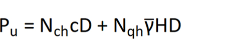
Where,
Maximum lateral soil force per unit length of pipe
Horizontal bearing capacity factor for clay (0 for c =0)
Horizontal bearing capacity factor for clay (0 for
Displacement at P
u=0.04(H+D/2) ≤ 0.10D to 0.15D
c) Vertical uplift soil springs
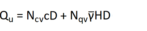
Where,
Maximum upward vertical soil force per unit length of pipe
Vertical uplift factor for clay (0 for c = 0)
Vertical uplift factor for sand (0 for Φ = 0)
0.01H to 0.02H for dense sands < 0.1D
0.1H to 0.2H for stiff to soft clays < 0.2D
d) Vertical bearing soil springs

Where,
Maximum vertical bearing soil force per unit length of pipe
Total unit weight of soil
The soil properties required for generating soil springs include the following parameters, which are typically obtained from geotechnical reports:
-
Soil type
-
Unit weight and effective unit weight of soil
-
Estimated water table level
-
Internal soil friction angle
-
Friction factor at the soil/pipe interface
-
Effective cohesion
-
Undrained shear strength
-
Soil adhesion factor
-
Coefficient of earth at rest
The typical soil properties for clay, sand, and gravel are listed below:
| Soil Type |
Bulk Unit Weight (kN/m3) |
Submerged Unit Weight (kN/m3) |
Undrained Shear Strength (kPa) |
Peak Effective Friction Angle (Deg) |
Effective Cohesion (kPa) |
| Stiff Clay |
19-21 |
9-11 |
40-100 |
25-30 |
0-10 |
| Soft Clay |
18-20 |
8-10 |
25-35 |
23-26 |
0-5 |
| Silty Sand - Loose |
18-19 |
8-9 |
0 |
26-30 |
0 |
| Gravel - Loose |
21-22 |
11-12 |
0 |
36-40 |
0 |
Soil spring stiffness significantly impacts the results of buried pipeline stress analysis; therefore, accurately calculating it is crucial for the success of the analysis. Attention should be given to the following issues:
-
Generally, backfill (disturbed) soil should be used to calculate axial soil spring stiffness. It is appropriate for calculating lateral and vertical uplifting soil spring stiffness only when it can be demonstrated that the extent of pipeline movement relative to the surrounding backfill soil is not influenced by the soils outside the pipe trench. Native (undisturbed) soil properties should be used for calculating vertical bearing spring stiffness.
-
For cohesive soils, such as clay, undrained shear strength should be utilized, with the friction angle typically set to 0. For non-cohesive soils, such as sand and gravel, drained soil parameters should be applied, using both the internal angle of friction and effective cohesion.
-
If an expansion medium, such as Ethafoam 220, is required, it should be modeled by either applying a stiffness coefficient for the expansion medium or removing the soil stiffness coefficient, thereby leaving a void where the expansion medium will be placed.
-
Organic soils can be assumed to be cohesive, with a lower undrained shear strength (e.g., 2.5 kPa to 5 kPa). The calculated yield displacement should be manually increased by 5 to 10 times in all directions using a soft clay coefficient value. The use of friction angle to calculate muskeg soil springs should be avoided, and the submerged density of the organic soil should be used for soil spring calculations.
-
Compaction levels significantly affect soil properties. A compaction level of over 95% is considered close to native soil conditions, while disturbed soils typically have compaction below 80%.
-
Water table levels are to be considered when developing soil springs. If there is available information to indicate that the water table is high, then the soil is considered to be submerged at that location, and the density parameter used in the soil spring calculation is to be modified. Otherwise, the dry density of the soil is to be used for the soil spring calculation.
4) Load and load combinations
Working loads to be considered in pipeline stress analysis typically include operating pressure, thermal expansion ranges, temperature differentials, sustained forces, and wind loads. Live loads, such as vehicle traffic, hydrostatic testing during pipeline filling, and the operation of cleaning pigs or inline inspection tools, are also included in the analysis.
Soil overburden and settlement are generally factored into the analysis as well. The soil overburden load due to backfill is calculated as a prism load per unit length using the following formula:
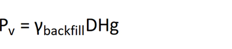
Where,
Load due to soil backfill (N)
Density of soil used for backfill (kg/m3)
Acceleration due to gravity, 9.8065 m/s2
Soil settlement, which is the downward movement of soil caused by factors such as the elastic rebound of the pipe, over-excavation of the ditch bottom, and inadequate compaction beneath large-diameter pipes, is treated as a working load in stress analysis. A typical assumption is a settlement of 25 mm for new buried piping segments and newly excavated sections of existing underground piping. This is simulated in the stress model by modifying the vertical soil spring to create a 25 mm displacement gap until the soil spring is engaged.
Soil Settlement Modelling
Additional loadings beyond those specified above include occasional extreme loads, such as inertial forces from earthquakes, slope movements, fault movements, seismic-related earth movements, thaw settlement, frost heave, and loss of support. These loads are typically not addressed in standards such as CSA Z662:23. However, it is important to assess whether supplemental design criteria are necessary for such loadings and whether additional strength or protection against damage modes, or both, should be provided.
The following table illustrates an example of load case combinations in AutoPIPE software per CSA Z662:23,
| Case No. |
Loadings |
Category |
CSA Z662 Clause |
Allowable |
| 1 |
Max P |
Hoop Stress |
Clause 4.3.5.1 |
SMYS x F x L x J x T |
| 2 |
HP |
Hydrotest |
Stresses due to hydrotest pressure |
1.25 x MOP |
| 3 |
GR + Max P |
Sustained Stress |
Stresses due to Sustained loads, Clause 4.8.5 |
SMYS x F x L x J x T |
| 4 |
Amb T to Max T |
Expansion Stress |
Thermal stress from minimum (or restraint) temperature to maximum temperature, Clause 4.8.4 |
0.72 x SMYS x T |
| Min T to Max T |
| 5 |
GR + Max P + U2 |
Occasional |
Stresses due to sustained loads and occasional load, Clause 4.8.5 |
SMYS x F x L x J x T |
| 6 |
GR + Max P + Max T |
Combined Stress |
Combined stress without bending, Clause 4.7.1 |
0.9 x SMYS x T |
| 7 |
GR + Max P + Max T |
Combined Stress |
Combined stress, Clause 4.7.2.1 |
1.0 x SMYS x T |
| 8 |
GR + Max P + Max T + U1 |
Combined Stress |
Combined stress with soil settlement, Cause 4.7.2.1 |
1.0 x SMYS x T |
| 9 |
GR + Max P + Max T + U1 + U2 |
Combined Stress |
Combined stress with soil settlement and occasional load, Clause 4.7.2.1 |
1.0 x SMYS x T |
Where,
GR – Weight of piping system due to gravity and soil overburden
HP – Hydrotest pressure
Max P – Maximum operating pressure (MOP)
Max T – Maximum operating temperature (may vary based on section of piping)
Min T – Minimum operating temperature (may vary based on section of piping)
Amb T – Ambient (or restraint) temperature
U1 – Soil settlement
U2 – Occasional loads (e.g., earthquake, wind, blowdown forces)
Verification of model involves validating the input data and performing a test run to ensure that the model accurately represents the real system.
Performing analysis includes calculating code stresses, displacements, and the overall behavior of the pipeline under various applied load cases. Code stresses typically include sustained stress, thermal expansion stress, occasional stress, and combined stress. Vertical displacements at overbends will be evaluated against specified limits to prevent upheaval buckling. Additionally, the following analyses are conducted to verify the stability and strength of the pipeline under special conditions:
Furthermore, stress analysis is also performed on pipeline assemblies and associated facilities piping.
Developing solutions is an iterative process that involves continuously modifying the pipeline system design until compliance with specified standards, typically CSA Z662 in Canada, is achieved.
When determining pipe stresses, the following concerns related to specific types of bends should be considered:
-
Side Bends: The pipeline is not fully restrained in the bend area; expansion at the bend will cause lateral soil reaction forces, resulting in bending stresses in the pipe.
-
Sag Bends: Bending and the resulting stresses at sag bends are typically not a concern, as the soil at the bottom of the ditch (outside of muskeg areas) is usually stiff.
-
Over Bends: The main concern with over bends is the potential for pipe buckling due to relatively weak restraining forces from the overburden.
-
Roping: The pipe will elastically deform as a beam under its own weight when placed in a ditch that is not perfectly straight. The roping bending radius should be calculated by limiting the bending stresses to 10% of the Specified Minimum Yield Strength (SMYS).
If high stress or significant bend movement is identified, the following mitigation methods should be considered to limit and reduce stress levels at bends:
-
Increase the bending radius.
-
Break up bends to occur over multiple joints.
-
Increase the depth of cover (if feasible) and/or modify backfill (if feasible).
-
Increase the wall thickness of the bend.
-
Increase the wall thickness and/or length of the pipe connected to each side of the bend.
-
Modify the pipe layout configuration,
-
Require selected trench backfilling and/or increased backfilling compaction,
-
Introduce or move the supports on the pipe system,
-
Change the pipe material.
Generating reports involves creating analysis result files that include the scope of work, analysis input data, code stress compliance, non-code analysis results, and recommendations (such as piping layout and support suggestions) for review.
Pipeline Stress Analysis Guidelines
(1) Governing codes and standards for pipeline stress analysis
Typical codes and standards applicable to pipeline stress analysis include, but not limited to:
-
CSA Z662 (Oil and Gas Pipeline Systems)
-
ASME B31.4 (Liquids and Slurries Pipeline), B31.8 (Gas Pipeline), B31.12 (Hydrogen Piping and Pipeline)
-
ASME Section VIII (Pressure Vessels)
-
API 610 (Centrifugal Pumps), API 676 (Positive Displacement Pumps), API 617 (Centrifugal Compressors), API 618 (Reciprocating Compressors), NEMA SM23/API 612 (Steam Turbines), API 661 (Air-Cooled Heat Exchangers), API 560 (Fired Heaters), API 650 (Flat Bottom Welded Storage Tanks)
(2) Allowable code stress limits
Each standard specifies different allowable limits for code stress corresponding to various load case combinations. For instance, according to CSA Z662:23, the allowable stress limits are summarized as follows:
a) The hoop stress for straight pipe is limited by:
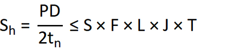
Where,
Pipe nominal wall thickness
Specified minimum yield strength
b) The combined hoop and longitudinal stresses for restrained portions of pipeline systems is limited by:
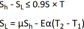
Where,
Hoop stress due to design pressure, MPa
Longitudinal compression stress, MPa
Modulus of elasticity of steel, MPa
Linear coefficient of thermal expansion, °C
-1
Maximum operating temperature, °C
Ambient temperature at time of restraint, °C
c) The combined stresses for restrained portions of pipeline systems is limited by:
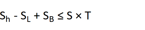
Where,
Hoop stress due to design pressure, MPa
Longitudinal compression stress, MPa
Absolute value of beam bending compression stresses resulting from live and dead loads, MPa
d) The stresses due to thermal expansion for unrestrained portions of pipeline systems is limited by:
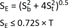
Where,
Thermal expansion stress range, MPa
Resultant bending stress from bending moment, MPa
Resultant torsional stress from torsional moment, MPa
e) The sum of the longitudinal pressure stress and the total bending stress due to sustained force and wind loading for unrestrained portions of pipeline systems is limited by:
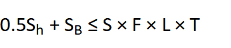
Where,
Hoop stress due to design pressure, MPa
Absolute value of beam bending compression stresses resulting from live and dead loads, MPa
Specified minimum yield strength, MPa
(3) Supplement design criteria
These criteria are typically specified by project specifications based on the applied loads and generally include the following:
a) Allowable uplift movement at bends
The allowable movement for bends from a previous project is as follows:
b) The bending moment on the hot tap branch side shall be limited to a specified value.
c) Local contact stresses caused by pipe supports on the pipe wall should be calculated to ensure there is no denting or yielding of the pipe wall due to support loadings.
d) Flange leakage must be checked in accordance with ASME VIII, Division 2.
Pipeline Stress Analysis Tools
Various analysis tools are available for pipeline stress analysis. At CCPGE, we utilize Bentley AutoPIPE and CAESAR II for this purpose. When necessary, we also employ Abaqus or ANSYS to address specific problems.
AutoPIPE and CAESAR II are widely recognized software applications for piping and pipeline stress analysis. They enable users to effectively create stress analysis models and define the loading conditions imposed on the system. Based on this input, the software generates results in the form of displacements, loads, and stresses throughout the system, comparing these results against limits specified by recognized codes and standards. Particularly, AutoPIPE features strong soil modeling capabilities, making it the preferred choice for conducting stress analysis on buried piping.
Abaqus is well-suited for complex nonlinear problems, including material nonlinearity, large deformations, and contact issues. Additionally, Abaqus provides tools for more accurately modeling the pipe-soil interface. These capabilities are essential for accurately simulating pipeline behavior under extreme conditions, such as buckling, collapse, or large displacements.
Buoyancy Control Analysis
What is Buoyance Control Analysis
Pipeline buoyancy control is required in areas with a high water table, lightweight backfill (such as muskeg or sugar sand), and water body crossings where the upward buoyant force acting on the pipeline exceeds the combined downward weight of the pipe and the soil column above it. Other locations, such as intermittently flooded areas (including irrigated fields, rice paddies, and river floodplains), may also require buoyancy control.
Pipeline buoyancy control analysis involves calculating buoyancy forces, determining the sizing and spacing of control measures, and assessing the resulting bending and membrane stresses against allowable limits. This analysis evaluates the most effective and appropriate buoyancy control measures to ensure that the pipeline remains in the desired position and maintains stability, thereby preventing issues such as floating or collapsing.
Buoyancy Forces on Pipe (Sourced from ALA 2001)
Why Perform Buoyance Control Analysis
Pipeline buoyancy control analysis optimizes the type, quantity, size, and spacing of buoyancy control measures based on site-specific conditions. This ensures that pipeline buoyancy is effectively managed throughout its lifecycle. The analysis also maintains bending and membrane stresses within allowable limits as specified by relevant codes and manufacturer specifications, thereby safeguarding pipe integrity and ensuring the operability of the system under all foreseeable conditions during both operations and construction.
Buoyance Control Analysis Methodology
(1) Buoyance control analysis procedure
a) Identify sections of pipeline that require buoyancy control
This is done by reviewing the pipeline Right of Way survey drawings and the geotechnical report to identify areas with muskeg, sugar sand, liquefiable soils, or other conditions that could affect buoyancy along the pipeline. If necessary, Ground Penetrating Radar (GPR) will be employed to confirm the depths of peat or swamp layers.
b) Perform buoyancy forces calculations
The buoyancy force imposed on a straight pipe can be calculated as follows:

Where,
Upward force due to buoyancy per unit length of pipe
Weight of water displaced by pipe per unit length of pipe
Weight of pipe per unit length of pipe
Weight of pipe contents per unit length of pipe
Height of fill above top of pipe
Height of water above pipe
Water buoyance factor = 1 - (hw /C)
A positive net buoyancy indicates that the pipe will float, while a negative value suggests it will sink. In cases where there is a net upward force, it is necessary to propose buoyancy control measures. Based on these calculations, the required weights for the buoyancy control measures will be determined. Additionally, the amount of contingency should take into account the reliability of site condition information and the minimum depth of cover required by code for buried pipelines.
c) Determine suitable buoyancy control measures for selected pipeline segments
Typical buoyancy control measures include continuous concrete coating (CCC), concrete swamp (saddle) weights, bolt-on (river) weights, screw anchors, and geotextile fabric weights (GFW). These measures are selected based on site-specific conditions. The following table provides a rule of thumb for this selection in some of past projects.
| Buoyancy Control Method |
Shallow Organics |
Deep Organics |
|
Typical Soil |
Typical Soil |
Shallow Bedrock |
Granular Soil |
Wet Organic Areas or Minor Water Crossings |
Major Water Crossings |
| Deeper Ditch |
✓✓ |
|
|
|
|
|
| Imported Fill |
✓ |
|
|
|
|
|
| Screw Anchors |
✓ |
✓✓ |
|
|
|
|
| Concrete Saddle Weights |
✓ |
✓ |
✓ |
✓ |
|
|
| Concrete Bolt-On Weights |
✓ |
✓ |
✓ |
✓ |
✓✓ |
|
| Geotextile Bag Weights |
✓ |
✓ |
✓✓ |
✓ |
|
|
| Concrete Coating |
|
✓ |
|
✓ |
✓ |
✓✓ |
| Notes: ✓✓ = Preferred option; ✓ = Optional |
The weights of the control measures will be strategically placed along the pipeline to ensure balance. The size (length and thickness) and spacing of these measures will be finalized based on the calculated piping stresses, including bending and membrane stress, resulting from buoyant upward forces and downward weight. It is essential that the calculated stresses for the designed sizes and spacing remain within allowable limits as specified by relevant standards during both construction and operation.
d) Perform buoyancy force re-calculations and pipeline bending and membrane stress check
Once the proposed buoyancy control measures are applied to the pipe, it is necessary to re-calculate the resultant forces, considering the weight, buoyancy, size (length and thickness), and spacing of the control measures. This ensures that the direction of the resultant force is downward, satisfying the negative buoyancy requirements, and that the calculated pipeline stresses comply with code requirements. If the conditions are not met, a redesign of the weights, size, and spacing of the control measures may be necessary, such as adjusting the spacing or thickness. This iterative process continues until both negative buoyancy and pipeline stress requirements are satisfied.
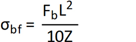
The bending stress induced in the pipe by buoyancy forces can be calculated according to ALA (2001) as follows:
Where,
Bending stress caused by buoyancy forces, Pa
Upward force due to buoyancy per unit length of pipe, N/m
Section modulus of the pipe cross-section, m3
Length of pipe span between two buoyancy control measures, m
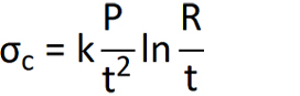
The membrane stresses developed as a result of the buoyancy force that pushes the pipe against the buoyancy control measures may be calculated using Roark - formula, as shown below.
Where,
Contact stress caused by buoyancy forces, N/m2
0.02−0.00012 (𝛽−90), unit-less
The calculated stresses will be combined with hoop stress, resulting from internal pressure, and longitudinal stress, caused by internal pressure and thermal effects. These combined stresses will then be compared against the allowable limits specified by applicable standards, such as CSA Z662:23.
e) Finding solution
Steps c) and d) will be repeated until satisfactory results are achieved, leading to the final solution for buoyancy control.
f) Documentation and reporting
This involves preparing comprehensive reports that detail the scope of work, input data, calculations, assumptions, design decisions, and recommendations for pipeline buoyancy control for review.
(2) Buoyancy control requirements
Buoyancy control calculations shall be performed for all types of buoyancy control measures to meet the specified negative buoyancy requirements. The following table presents an example used in previous projects.
| Type |
Percentage of Negative Buoyancy |
| Watercourse Crossings |
10% |
| Wetlands |
5% |
| Screw Anchors |
0% |
Notes on Buoyancy Control Analysis
Buoyancy control analysis is typically conducted alongside pipeline stress analysis. The proposed buoyancy control measures will be integrated into stress models, particularly during the lowering-in analysis, resulting in a cohesive design.
Upheaval Buckling Analysis
What is Buckling Analysis
Pipeline buckling refers to the deformation of a pipeline caused by compressive forces that exceed the structural capacity of the pipe, leading to over bending or collapse. Buckling is usually not an issue for buried pipelines in competent soil, but it can be a serious concern when the pipeline is in muskeg areas.
Pipeline upheaval buckling analysis involves evaluating the stability of pipelines that may undergo upward deformation due to various applied loads. This analysis provides insights into the critical conditions under which buckling may occur, including load thresholds and potential deformations.
Pipeline Upheaval Buckling
Why Perform Buckling Analysis
Pipeline upheaval buckling analysis evaluates the risk of buckling in pipelines caused by axial loads, lateral forces, temperature changes, soil movement, and more. This analysis defines the minimum required cover depth and the maximum height of soil profile imperfections that could lead to an overbend at the top of the trench. By performing this analysis, the following risks can be mitigated:
-
Loss of pipeline structural integrity
-
Pipeline leakage due to excessive deformation
-
Operational downtime from repairing or replacing buckled sections of the pipeline
In summary, pipeline upheaval buckling analysis is a critical process for ensuring the structural integrity and safety of pipeline systems, particularly in challenging environments and under varying operational conditions.
Upheaval Buckling Analysis Methodology
Two types of buckling analysis, one for straight pipe and one for overbends, are typically required, each using different methods.
(1) Straight pipe - Troitsky analysis
Troitsky’s analysis involves determining the critical buckling force by assuming a straight, elastic pipeline of infinite length. The total longitudinal compressive force in the pipeline, resulting from hoop stress and thermal differentials, is also calculated. The pipeline is considered stable if 110% of the compressive force is less than the critical buckling force.
The analysis steps are outlined as follows
Step 1: Calculate the axial resistance to pipe movement by the following formula
p = πDc + 0.8tan(1.6ρgHD + 0.9q1g), for sandy and dry clayey soils:
p = πDc + tan(1.6ρgHD + 0.9qq1g), for clayey soils:
Where,
Height of fill above pipe, m
Outer diameter of pipe, m
Mass per unit length of the pipe, kg/m
Step 2: Calculate the transverse resistance to pipe movement by the following formula
Where,
Transverse resistance, N/m
Angle of internal friction of soil, rad
Depth to center of the pipe, m
Step 3: Calculate the critical buckling load by the following formula
Where,
Critical buckling load, N
Cross-section area of the pipe, m
2
Modulus of elasticity, Pa
Step 4: The axial compressive force is calculated by the following formula:
[(1 - 2ν)P
MOPA
i + EαA(T
d - T
i)]
Where,
Axial compressive force, N
Design or maximum operating pressure, N/m
2
Internal area of pipe, m
2
Coefficient of thermal expansion, °C
-1
Installation temperature, °C
Step 5: The pipe is considered to be stable if the following condition is true:
(2) Straight Pipe - Hobbs Analysis
This analysis is based on the technical paper "In-Service Buckling of Heated Pipelines," which discusses both vertical and lateral buckling. The method involves the following steps:
Step 1: Calculate co-efficient of friction by using the soil friction angle provided in the geotechnical report.
Where,
Soil friction angle, degree
Step 2: Calculate the buckle length at minimum axial load using the following equation

Where,
Modulus of elasticity, Pa
Area modulus of section, m
4
Linear weight of complete pipe system, N/m
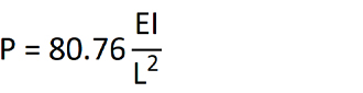
Step 3: Calculate axial load in the buckle as follows:
Where,
Buckle length at minimum axial load, m
Step 4: Calculate axial load away from the buckle P0 by the formula

Where,
Axial load away from the buckle, N.
Step 5: Calculate the maximum temperature differential by the following formula

Where,
Maximum temperature differential, °C
Coefficient of thermal expansion, °C
-1
Step 6: Using a range of multipliers of the buckle length at minimum axial load L, from 0.5L to 3.0L in increments of 0.1, calculate the maximum temperature differential by repeating the above steps. Develop a graph with the buckling length on the x-axis and calculated temperature differential on the y-axis to find the lowest value of temperature differential. That value represents the largest safe temperature differential for which the pipeline will not buckle. If this allowable temperature differential is more than the design temperature differential, then upheaval buckling is not a concern per the Hobbs method.
(3) Overbends - Parametric studies
For overbends with smaller cold field bend angles (typically less than 8° to 10°) that have not been accurately identified along the pipeline right-of-way and, therefore, not included in the pipeline stress analysis model, parametric studies are necessary to assess potential upheaval buckling. These studies will investigate stresses and displacements at these overbends to ensure they remain within defined allowable limits.
Overbends exhibiting high displacement and/or stresses exceeding allowable limits must be mitigated using various control methods. Options include the installation of screw anchors as the primary solution in organic soil sections, increased burial depth as the primary method in mineral soil sections, and increasing the bending radius where necessary. Geotextile Fabric Weights (GFW) may be utilized in locations where screw anchor installation is not feasible
AutoPIPE software can be utilized for parametric studies of overbends. Models can be created to simulate overbends across a range of angles, with mitigation forces evenly distributed over the bends.
(4) Overbends - Palmer Method
Palmer method can be used for buckling calculations of pipes with a geometrical imperfection. The imperfection can be a measure of a bend. The method involves the following steps:
Step 1: Calculate the axial load due to pressure and thermal extension

Where,
Axial load due to pressure and thermal extension, N
Cross sectional area of pipe, mm
2
Modulus of elasticity, Pa
Maximum operating temperature, °C
Ambient temperature at time of restraint, °C
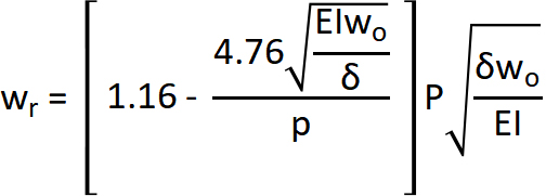
Step 2: Calculate required downward force for stability in operating condition
Where,
Required downward force for stability in operating condition, N/mm
Imperfection height (use 0.01 to represent 1 straight pipe, mm
Pipe moment of inertia, mm
4
Modulus of elasticity, Pa
Axial load due to pressure and thermal expansion, N
Installation weight of pipe, N/mm
Step 3: Calculate Available Downward Force
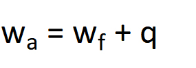
Where,
HDγ
soil(1 - f(H/D)) for cohesionless sand, silt and rock, and q = cDmin [3,H/D] for cohesive clay and silt
Available downward force for stability in operating condition, N/m
Operating weight of pipe, N/m
Uplift resistance of cover, N/m
Outside diameter of pipe, m
Uplift coefficient, 0.50 for dense materials and 0.10 for loose material
Unit weight of cover material, N/m
3
Step 4: Compare the available downward force to the required downward force to assess the risk of buckling
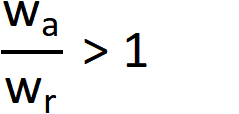
Where,
Available downward force for stability in operating condition, N/m
Required downward force for stability in operating condition, N/m
If the available load divided by the required load is greater than one, then the amount of cover provided is sufficient to withstand pipe buckling.
Notes on Upheaval Buckling Analysis
-
Analysis methods: Traditional formulas and equations can be used to predict buckling behavior based on pipe dimensions and material properties. For more complicated cases, a Finite Element Analysis (FEA) method is usually used to simulate the behavior of the pipeline under various loads and conditions.
-
Acceptable limits: Compliance with relevant industry standards that provide guidelines for buckling analysis and acceptable limits.